Kappa
“Great things are not done by impulse, but by a series of small things brought together.”
Hack The Box
Q-Learning
Q-learning is a model-free reinforcement learning algorithm that learns an optimal policy by estimating the Q-value. The Q-value represents the expected cumulative reward an agent can obtain by taking a specific action in a given state and following the optimal policy afterward. It's called "model-free" because the agent doesn't need a prior model of the environment to learn; it learns directly through trial and error, interacting with the environment and observing the outcomes.
Imagine a self-driving car learning to navigate a city. It starts without knowing the roads, traffic lights, or pedestrian crossings. Through Q-learning, the car explores the city, taking actions (accelerating, braking, turning) and receiving rewards (for reaching destinations quickly and safely) or penalties (for collisions or traffic violations). Over time, the car learns which actions lead to higher rewards in different situations, eventually mastering the art of driving in that city.
The Q-Table
At the heart of Q-learning lies the Q-table. This table is a core algorithm component, storing the Q-values for all possible state-action pairs. Think of it as a lookup table that guides the agent's decision-making process. The rows of the table represent the states (e.g., different locations in the city for the self-driving car), and the columns represent the actions (e.g., accelerate, brake, turn left, turn right). Each cell in the table holds the Q-value for taking a particular action in a particular state.
Below is an illustration of a simple Q-table for a grid world environment where a robot can move up, down, left, or right. The grid cells represent the states, and the actions are the possible movements.
          State/Action  Up      Down    Left    Right
          ------------  ----    ----    ----    -----
          S1            -1.0    0.0     -0.5    0.2
          S2            0.0     1.0     0.0     -0.3
          S3            0.5     -0.5    1.0     0.0
          S4            -0.2    0.0     -0.3    1.0
In this table, S1, S2, S3, and S4 are different states in the grid world. The values in the cells represent the Q-values for taking each action from each state.
The Q-value for a particular state-action pair is updated using the Q-learning update rule, which is based on the Bellman equation:
          Q(s, a) = Q(s, a) + α * [r + γ * max(Q(s', a')) - Q(s, a)]

          Where:
            Q(s, a) is the current Q-value for taking action a in state s.
            α (alpha) is the learning rate, which determines the weight given to new information.
            r is the reward received after taking action a from state s.
            γ (gamma) is the discount factor, which determines the importance of future rewards.
            max(Q(s', a')) is the maximum Q-value of the next state s' and any action a'.
Let's use an example of updating a Q-value for the robot in the grid world environment.
- The robot is currently in state S1.
- It takes action Right, moving to state S2.
- It receives a reward r = 0.5 for reaching state S2.
- The learning rate α = 0.1.
- The discount factor γ = 0.9.
- The maximum Q-value of the next state S2 is max(Q(S2, Up), Q(S2, Down), Q(S2, Left), Q(S2, Right)) = max(0.0, 1.0, 0.0, -0.3) = 1.0.
Using the Q-learning update rule:
          Q(S1, Right) = Q(S1, Right) + α * [r + γ * max(Q(S2, a')) - Q(S1, Right)]
          Q(S1, Right) = 0.2 + 0.1 * [0.5 + 0.9 * 1.0 - 0.2]
          Q(S1, Right) = 0.2 + 0.1 * [0.5 + 0.9 - 0.2]
          Q(S1, Right) = 0.2 + 0.1 * 1.2
          Q(S1, Right) = 0.2 + 0.12
          Q(S1, Right) = 0.32
After updating, the new Q-value for taking action Right from state S1 is 0.32. This updated value reflects the robot's learning from the experience of moving to state S2 and receiving a reward.
The Q-Learning Algorithm
The Q-learning algorithm is an iterative process of action selection, observation, and Q-value updates. The agent continuously interacts with the environment, learning from its experiences and refining its policy to maximize cumulative rewards.
Here's a breakdown of the steps involved:
- Initialization: - The Q-table is initialized, typically with arbitrary values (e.g., all zeros) or with some prior knowledge if available. This table will be updated as the agent learns.
- Choose an Action: - In the current state, the agent selects an action to execute. This selection involves balancing exploration (trying new actions to discover potentially better strategies) and exploitation (using the current best-known action to maximize reward). This balance ensures that the agent explores the environment sufficiently while capitalizing on existing knowledge.
- Take Action and Observe: - The agent performs the chosen action in the environment and observes the consequences. This includes the new state it transitions to after taking the action and the immediate reward received from the environment. These observations provide valuable feedback to the agent about the effectiveness of its actions.
- Update Q-value: - The Q-value for the state-action pair is updated using the Q-learning update rule, which incorporates the received and estimated future rewards from the new state.
- Update State: - The agent updates its current state to the new state it transitioned to after taking the action. This sets the stage for the next iteration of the algorithm.
- Iteration: - Steps 2-5 are repeated until the Q-values converge to their optimal values, indicating that the agent has learned an effective policy, or a predefined stopping condition is met (e.g., a maximum number of iterations or a time limit).
This iterative process allows the agent to continuously learn and refine its policy, improving its decision-making abilities and maximizing its cumulative rewards over time.
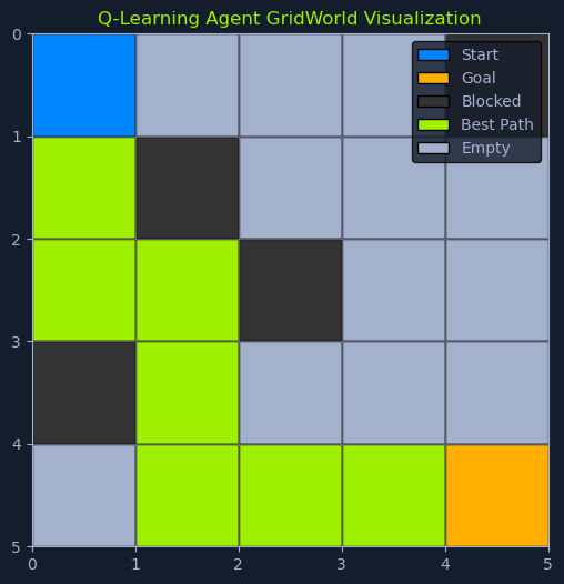
Ultimately, the agent successfully navigates from the start to the goal by following the path that maximizes the cumulative reward.
Exploration-Exploitation Strategy
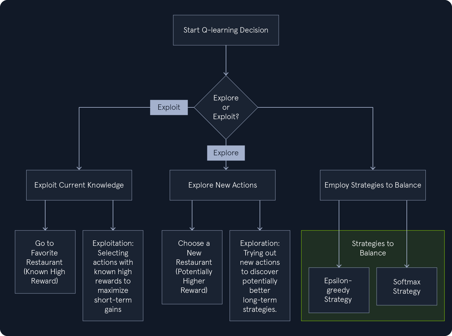
In Q-learning, the agent faces a fundamental dilemma: Should it explore new actions to discover better strategies potentially, or should it exploit its current knowledge and choose actions that have yielded high rewards in the past? This is the exploration-exploitation trade-off, a crucial aspect of reinforcement learning.
Think of it like choosing a restaurant for dinner. You could exploit your existing knowledge and go to your favorite restaurant, where you know you'll enjoy the food. Or, you could explore a new restaurant, taking a chance to discover a hidden gem you might like even more.
Q-learning employs various strategies to balance exploration and exploitation. The goal is to find a balance that allows the agent to learn effectively while maximizing its rewards.
- Exploration: - Encourages the agent to try different actions, even if they haven't previously led to high rewards. This helps the agent discover new and potentially better strategies.
- Exploitation: - This strategy focuses on selecting actions that have previously resulted in high rewards. It allows the agent to capitalize on existing knowledge and maximize short-term gains.
Epsilon-Greedy Strategy
The epsilon-greedy strategy offers a simple yet effective approach to balancing exploration and exploitation in Q-learning. It introduces randomness into the agent's action selection, preventing it from always defaulting to the same actions and potentially missing out on more rewarding options.
The epsilon-greedy strategy encourages you to explore new options while still allowing you to enjoy your known favorites. With probability epsilon (ε), you venture out and try a random coffee shop, potentially discovering a hidden gem. With probability 1-epsilon, you stick to your usual spot, ensuring a satisfying coffee experience.
The value of epsilon is a key parameter that can be adjusted over time to fine-tune the balance between exploration and exploitation.
- High Epsilon (e.g., 0.9): - A high epsilon value initially promotes more exploration. This is like being new in town and eager to try different coffee shops to find the best one.
- Low Epsilon (e.g., 0.1): - As you gain more experience and develop preferences, you might decrease epsilon. This is like becoming a regular at your favorite coffee shop while occasionally trying new places.
Data Assumptions
Q-learning makes minimal assumptions about the data:
- Markov Property: - It assumes that the environment satisfies the Markov property, meaning that the next state depends only on the current state and action, not on the history of previous states and actions.
- Stationary Environment: - It assumes that the environment's dynamics (transition probabilities and reward functions) do not change over time.
Q-learning is a powerful and versatile algorithm for learning optimal policies in reinforcement learning problems. Its ability to learn without a model of the environment makes it suitable for a wide range of applications where the environment's dynamics are unknown or complex.
Fundamentals of AI
- Introduction to Machine Learning
- Mathematics Refresher for AI
- Supervised Learning Algorithms
- Linear Regression
- Logistic Regression
- Decision Trees
- Naive Bayes
- Support Vector Machines (SVMs)
- Unsupervised Learning Algorithms
- K-Means Clustering
- Principal Component Analysis (PCA)
- Anomaly Detection
- Reinforcement Learning Algorithms
- ~ Q-Learning
- SARSA (State-Action-Reward-State-Action)